How To: Scraping MLB Free Agent Data

Building tables and plots using data from spotrac and Fangraphs

Good morning! In case you missed it, we’re now posting tutorials on how to make some of the tables and graphics contained in the newsletter. These posts will be for premium subscribers only, but we’ll occasionally post them for everyone like we did last week. You can find that post here. Today, we’ll recreate some of the tables from yesterday’s post where we looked at the upcoming free agent class.

Important note: The tutorial posts are going to assume that the reader has at least a basic understanding of R. If you’ve never written a line of code or worked with baseball data, there are many great introductory resources out there. A great place to start is R for Data Science by Hadley Wickham & Garrett Grolemund. It covers everything you’ll need to know to begin working with data, performing analysis, and building visualizations. RStudio also puts out many great resources like this guide for getting started in R. In our tutorials we’ll strictly be using baseball data, which in our opinion, makes it more fun to learn how to write code in R.

If you are a premium subscriber and don’t care about R or coding, you can skip past this section and go right to the updates from the Arizona Fall League last night.

---

Scraping Free Agent Data from Spotrac

UPDATE 12/2: The Spotrac page has changed, so the current iteration of this code won’t work. The basic ideas remain, but if you simply copy and paste the code it won’t work. We’ll update the code as soon as possible!

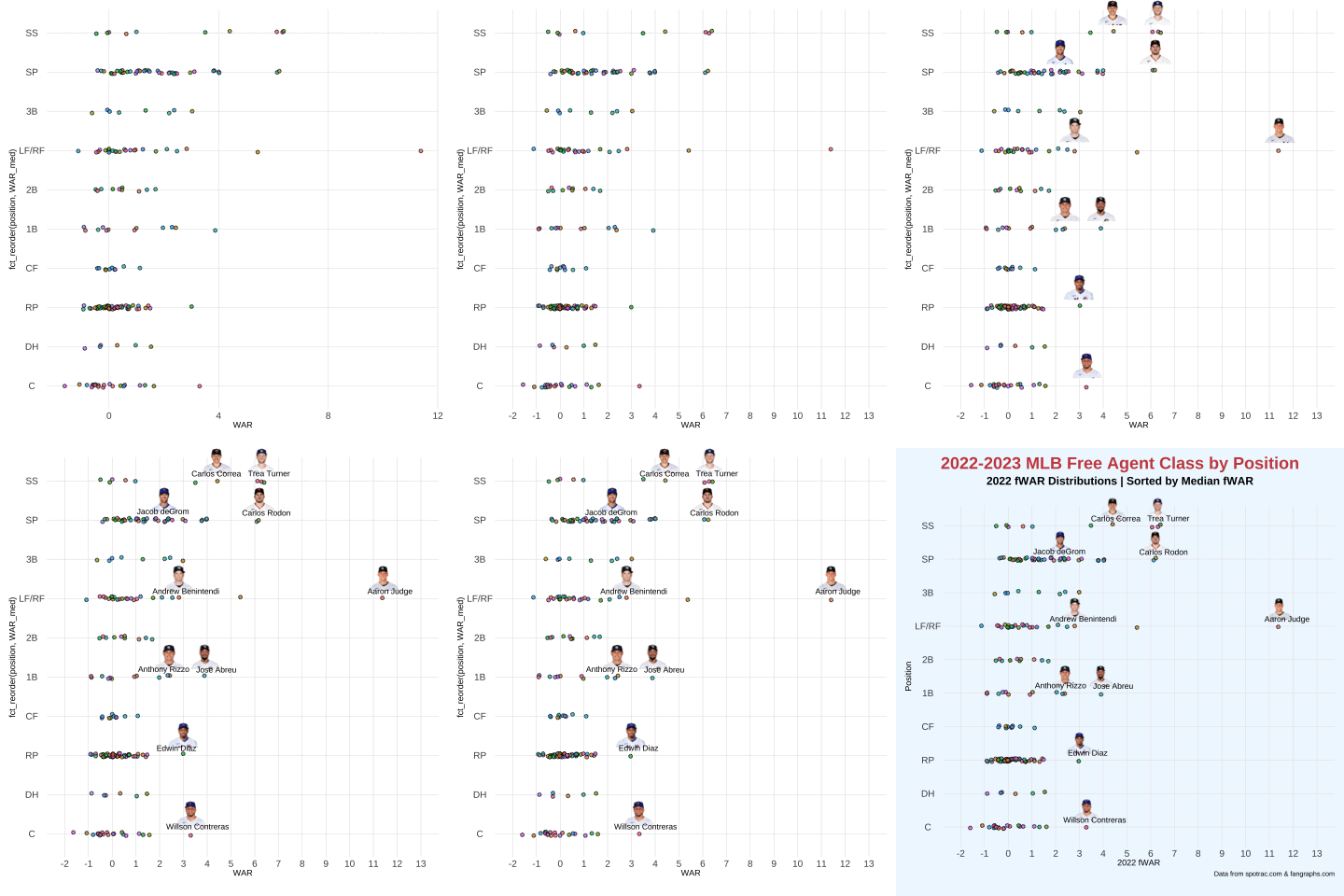
Today we’re going to take a look at the upcoming MLB free agent class by scraping some data from the spotrac.com. Spotrac does a nice job of compiling player contract and transaction data across all major sports, including baseball. We’ll then take the spotrac data and combine it with some stats from Fangraphs. We’ll use our data to construct a few nice looking tables and build a plot looking at the distribution of 2022 fWAR by position for this year’s free agent class.

As usual, the first thing we have to do is load up any packages we need and set a custom theme for the plot we’re going to build later.

# Load packages
library(tidyverse)
library(rvest)
library(baseballr)
library(data.table)
library(stringr)
library(mlbplotR)
library(ggrepel)
library(gt)
library(gtExtras)

# set custom theme for plot
theme_scott <- function () {

    theme_minimal(base_size=9) %+replace%
    theme(
        panel.grid.minor = element_blank(),
        plot.background = element_rect(
            fill = "aliceblue", color = "aliceblue"
        ),
        axis.text.y = element_text(size = 10),
        axis.text.x = element_text(size = 10),
       plot.margin = margin(10, 10, 20, 10) 
    )

}

Now we can start grabbing data. Because this page on spotrac has the free agent data in a table already, it’s pretty simple to scrape it using the rvest package. We’re actually going to do this in two steps. The reason is that if we just grab the entire table the player names are not in an easy to use form. They read something like this - “deGromJacob deGrom”. We could pull apart the names in this column, but it starts to get messy when you have names that don’t easily conform to a consistent pattern, such as “Bradley Jr.Jackie Bradley Jr.”. Instead, we’ll grab the player column separately from the table and parse only the text for the full name. After that, we can just bind that new column to our existing dataframe.